How To Find Duplicates In Excel Column

How to Notice Duplicates in Excel?

In MS Excel, the duplicate values tin be found and removed from a information set. Depending on your data and requirement, the most commonly used methods are the conditional formatting feature or the COUNTIF formula to observe and highlight the duplicates for a specific number of occurences. The columns of the data set can exist and so filtered to view the duplicate values.

In this article, we will wait at v different methods to cheque, identify, and delete duplicates in Excel.

5 Methods to Cheque & Identify Duplicates in Excel

You lot can download this Find for Duplicates Excel Template hither – Find for Duplicates Excel Template

#1 – Conditional Formatting

The conditional formatting Provisional formatting is a technique in Excel that allows us to format cells in a worksheet based on certain conditions. It can be establish in the styles section of the Home tab. read more feature is bachelor in Excel 2007 and subsequent versions.

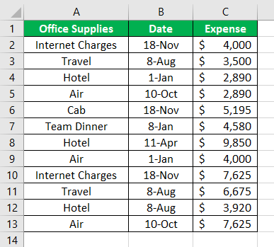
The post-obit tabular array consists of the expenses incurred on availing certain role facilities. The corresponding dates of purchasing such facility are also listed.

We want to identify the duplicates in excel with the help of provisional formatting.

The steps to discover the duplicates in excel with the assist of conditional formatting are listed as follows:

1. Select the data range (A1:C13) where duplicates are to be found.
2. In the Habitation tab, select "conditional formatting" from the "styles" section. From the driblet-down menu, select "highlight cell rules" and click on "duplicate values."

   
   

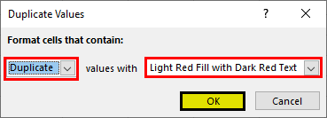
3. The pop-upwards window titled "duplicate values" appears. In the beginning box on the left side, select "indistinguishable." In the "values with" drop-down, select the required color to highlight the duplicate cells. Click "Ok."

   
   

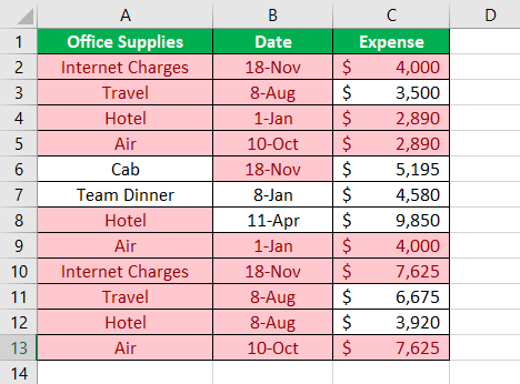
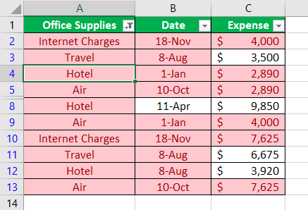
4. The duplicate cells are highlighted in the data table, as shown in the following image.

   
   

5. The columns can be filtered to identify the duplicate values. For this, right-click the required column and select "filter by selected prison cell's colour." The information is filtered for duplicates.

   
   

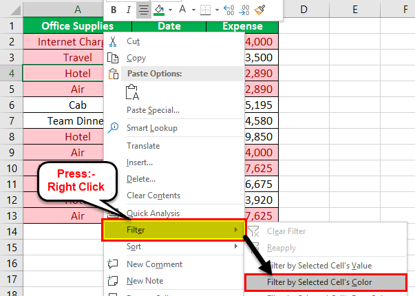
6. The result after applying the filter to the first cavalcade (role supplies) is shown in the post-obit image.

   
   

#2 – Conditional Formatting (Specific Occurrence)

Permit us consider an example to identify the specific number of duplications. In the following table, we want to check and prove the indistinguishable values with iii occurrences.

The steps to find the indistinguishable values for specific number of occurrences are listed as follows:

Step 1: Select the range A2:C8 in the given data table.

Pace 2: In the Home tab, select "provisional formatting" from the "styles" section. Click "new rule."

Note: The "new rule" choice helps highlight a specific count of duplicates using the COUNTIF formula.

Step three: The popular-up window titled "new formatting rule" appears. Enter the following details, every bit shown in the succeeding prototype.

• Under "select a rule type," select "use a formula to decide which cells to format."
• Under "edit the rule description," enter the COUNTIF The COUNTIF function in Excel counts the number of cells within a range based on pre-defined criteria. It is used to count cells that include dates, numbers, or text. For case, COUNTIF(A1:A10,"Trump") volition count the number of cells within the range A1:A10 that contain the text "Trump" read more formula.

The COUNTIF formula "=COUNTIF(cell range of the data table, cell criteria)" finds and highlights the cells for the desired number of occurrences.

In this case, the COUNTIF formula highlights duplicate cells having triplicate count. This count tin can be inverse to a greater number. The conditions can too be inverse depending on the user's requirement.

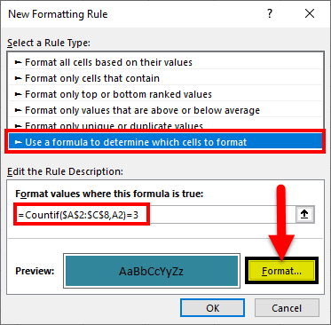
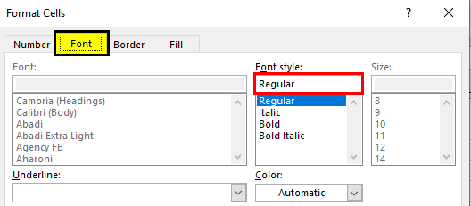
Step iv: In one case the COUNTIF formula is entered, click "format." The popular-up window titled "format cells" opens. Select the font style "regular."

Pace 5: In the "fill" tab, select blue color. The "fill" tab helps highlight the duplicate cells Highlight Cells Rule, which is bachelor under Conditional Formatting under the Home menu tab, can be used to highlight duplicate values in the selected dataset, whether information technology is a column or row of a table. read more .

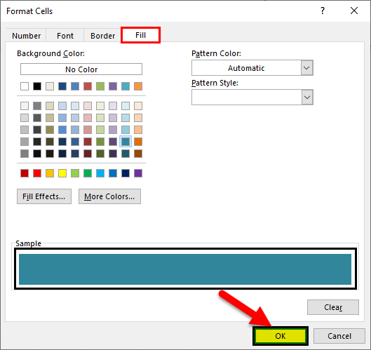
Step vi: Once the selections in "format cells" window are consummate, click "Ok." Click "Ok" once more in the "new formatting rule" window.

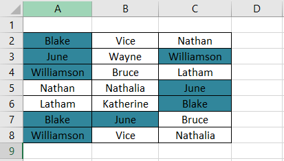
Stride 7: The result is displayed in the post-obit image. The duplicate cells with three occurrences are highlighted.

#three – Alter Rules (Formulas)

Working on the data of case #2, let us understand the procedure of changing the formula. For applying new formulas, the existing rules (formulas) of the information table A data table in excel is a type of what-if analysis tool that allows yous to compare variables and see how they impact the result and overall data. It tin can be found nether the data tab in the what-if analysis section. read more accept to be cleared.

The steps to clear the existing rules (shown in the succeeding image) are listed as follows:

Step 1: In the Home tab, select "conditional formatting" from the "styles" department.

Step 2: In "clear rules" option, select either of the following:

• Clear rules from selected cells–This resets the rules for the selected range of the tabular array. And then, prior to clearing the rules, the data needs to be selected.
• Articulate rules from unabridged canvas–This clears the rules for the unabridged sheet.

The bluish highlighted cells disappear and the original table is displayed.

#four – Remove Duplicates

Let united states check and delete duplicate values from a selected range. Prior to deletion, keeping a copy of  the tabular array is appropriate considering the duplicates will exist permanently deleted.

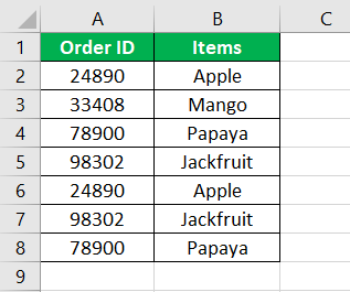
The following table displays a series of items with their corresponding IDs.

The steps to observe and delete indistinguishable values are listed as follows:

Pace 1: Select the range of the table whose duplicates are required to exist deleted.

Pace two: In the Information tab, select "remove duplicates" from the "data tools" section.

Notation: The "remove duplicates" option helps eliminate duplicates and retain unique cell values.

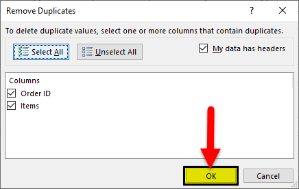
Step 3: The pop-upwardly window titled "remove duplicates" appears, as shown in the succeeding image. By default, the following options are already selected:

• The checkboxes for both the headers ("order ID" and "items")
• The "select all" box

Since the table consists of column headers, select the checkbox "my data has headers." Click "Ok" to execute.

Note: To change the number of columns selected, click "unselect all."  Following this, the desired columns from which the duplicates are to be deleted can be selected.

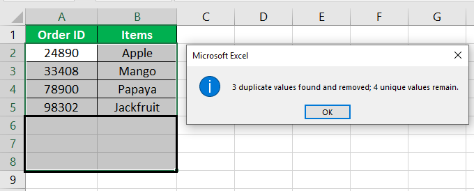
Step 4: The result is shown in the succeeding image. A prompt is displayed which states the following details:

• The number of indistinguishable values removed from the table
• The number of unique values that remain in the tabular array after deletion

Click "Ok." Hence, the duplicate values along with their respective rows are deleted.

#v – COUNTIF Formula

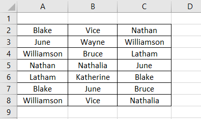
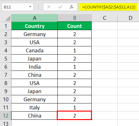
The following table displays the names of a few countries. We want to identify the duplicate values using the COUNTIF function.

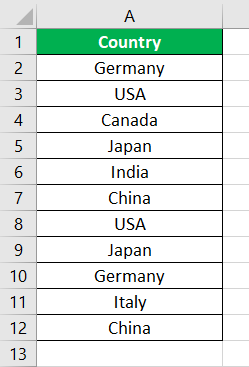
The COUNTIF function requires the range (cavalcade containing duplicate entries) and the cell criteria. It returns the number of corresponding duplicates for every cell.

The steps to find the duplicate values in excel with the assistance of the COUNTIF office are listed as follows:

Step 1: Enter the formula shown in the succeeding prototype. Press the "Enter" key.

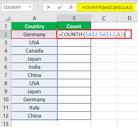
Note: The range must be stock-still with the dollar ($) sign. Otherwise, the cell reference volition modify on dragging the formula.

Stride 2: Drag the formula till the cease of the table with the help of the make full handle. Alternatively, identify the cursor on jail cell B2 and double-click the fill handle. The fill handle appears at the lower correct corner of cell B2.

Step 3: The output of the formula is shown in the following prototype. Information technology returns the count of duplicates for the unabridged data fix.

Note: The filter can be practical to the column header to view the occurrences greater than ane.

Frequently Asked Questions

1. What does it hateful to find duplicates in Excel?

While consolidating different worksheets, several duplicates may exist constitute in a data set. MS Excel helps to detect and highlight such duplicates. It is as well possible to filter a cavalcade for duplicate values.

An easy style to search for duplicates is past using the COUNTIF formula. This formula can count the total number of duplicates in a column. It tin likewise count the number of private instances of a particular indistinguishable entry. It accepts two arguments–the range and the criteria.

2. How to find duplicates in a column of Excel?

To check a column for duplicates, the formula is given as follows:

"=COUNTIF(A:A,A2)>1"

The formula checks for duplicates in column A. The topmost cell is A2. For every duplicate value, the formula returns "true." For every unique value, the formula returns "false."

Note: For an output other than "truthful" and "simulated," the COUNTIF formula tin exist enclosed in the IF function.

3. What is the formula to notice duplicates in Excel?

The generic formula to notice the exact, instance-sensitive duplicate values is stated as follows:
"IF(SUM((-Verbal(range,uppermost_cell)))<=ane,"","Duplicate")"

The EXACT function compares the cell range with the target jail cell. The SUM part adds the number of instances. If the occurrence is greater than one, the IF function returns "duplicate."
Note one: Since it is an array formula, it should be entered using "Ctrl+Shift+Enter."

Note 2: If the same word appears twice in lowercase and in one case in upper-case letter, the formula will not count the uppercase word every bit indistinguishable.

Recommended Manufactures

This has been a guide to Find Duplicates in Excel. Here we discuss how to identify, cheque and show duplicates in excel with examples. You lot may too look at these useful functions in Excel –

• How to Utilize IF Formula in Excel (with Examples)?
• Provisional Formatting for Blank Cells | Steps
• Create a Dashboard in Excel
• Apply Conditional Formatting in Pivot Table

• 35+ Courses
• 120+ Hours
• Full Lifetime Access
• Certificate of Completion

Learn MORE >>

Source: https://www.wallstreetmojo.com/find-duplicates-in-excel/

Posted by: kellumexclout.blogspot.com

Share this post